numpy.random.RandomState.standard_t

method

random.RandomState.standard_t(df, size=None)

Draw samples from a standard Student’s t distribution with df degrees of freedom.

A special case of the hyperbolic distribution. As df gets large, the result resembles that of the standard normal distribution (standard_normal).

Note

New code should use the standard_t method of a default_rng() instance instead; please see the Quick Start.

Parameters

dffloat or array_like of floats

Degrees of freedom, must be > 0.

sizeint or tuple of ints, optional

Output shape. If the given shape is, e.g., (m, n, k), then m * n * k samples are drawn. If size is None (default), a single value is returned if df is a scalar. Otherwise, np.array(df).size samples are drawn.

Returns

outndarray or scalar

Drawn samples from the parameterized standard Student’s t distribution.

See also

Generator.standard_t

which should be used for new code.

Notes

The probability density function for the t distribution is

\[P(x, df) = \frac{\Gamma(\frac{df+1}{2})}{\sqrt{\pi df} \Gamma(\frac{df}{2})}\Bigl( 1+\frac{x^2}{df} \Bigr)^{-(df+1)/2}\]

The t test is based on an assumption that the data come from a Normal distribution. The t test provides a way to test whether the sample mean (that is the mean calculated from the data) is a good estimate of the true mean.

The derivation of the t-distribution was first published in 1908 by William Gosset while working for the Guinness Brewery in Dublin. Due to proprietary issues, he had to publish under a pseudonym, and so he used the name Student.

References

1

Dalgaard, Peter, “Introductory Statistics With R”, Springer, 2002.

2

Wikipedia, “Student’s t-distribution” https://en.wikipedia.org/wiki/Student’s_t-distribution

Examples

From Dalgaard page 83 [1], suppose the daily energy intake for 11 women in kilojoules (kJ) is:

>>> intake = np.array([5260., 5470, 5640, 6180, 6390, 6515, 6805, 7515, \
...                    7515, 8230, 8770])

Does their energy intake deviate systematically from the recommended value of 7725 kJ? Our null hypothesis will be the absence of deviation, and the alternate hypothesis will be the presence of an effect that could be either positive or negative, hence making our test 2-tailed.

Because we are estimating the mean and we have N=11 values in our sample, we have N-1=10 degrees of freedom. We set our significance level to 95% and compute the t statistic using the empirical mean and empirical standard deviation of our intake. We use a ddof of 1 to base the computation of our empirical standard deviation on an unbiased estimate of the variance (note: the final estimate is not unbiased due to the concave nature of the square root).

>>> np.mean(intake)
6753.636363636364
>>> intake.std(ddof=1)
1142.1232221373727
>>> t = (np.mean(intake)-7725)/(intake.std(ddof=1)/np.sqrt(len(intake)))
>>> t
-2.8207540608310198

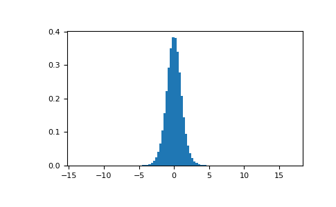
We draw 1000000 samples from Student’s t distribution with the adequate degrees of freedom.

>>> import matplotlib.pyplot as plt
>>> s = np.random.standard_t(10, size=1000000)
>>> h = plt.hist(s, bins=100, density=True)

Does our t statistic land in one of the two critical regions found at both tails of the distribution?

>>> np.sum(np.abs(t) < np.abs(s)) / float(len(s))
0.018318  #random < 0.05, statistic is in critical region

The probability value for this 2-tailed test is about 1.83%, which is lower than the 5% pre-determined significance threshold.

Therefore, the probability of observing values as extreme as our intake conditionally on the null hypothesis being true is too low, and we reject the null hypothesis of no deviation.

numpy.random.RandomState.standard_normal numpy.random.RandomState.triangular